Example of data visualization and exploration report
Speed dating data
This report was submitted by a group of students as part of the course MATH-517 at EPFL, and is presented here as an example of a data visualization and exploration.
Introduction
In a contemporary society characterized by fleeting moments and limited time, the concept of speed dating has emerged as a compelling avenue for those seeking to forge romantic connections : but what are its underlying dynamics ? Are there gendered differences in partner preferences ? How much do shared interests and ethnicity preferences affect compatibility ? What sets apart successful and unsuccessful candidates ? This report presents an analysis of the data associated to the Speed dating dataset used in Fisman et al. (2006). As we navigate through the nuanced world of speed dating, we uncover the data-driven insights that shed light on how these factors shape the pursuit of love within brief encounters.
Data description
The dataset was compiled by Columbia Business School professors Ray Fisman and Sheena Iyengar for their paper Gender Differences in Mate Selection: Evidence From a Speed Dating Experiment.
Data was gathered from participants in experimental speed dating events from 2002-2004. During the events, the attendees would have a four minute “first date” with every other participant of the opposite sex. At the end of their four minutes, participants were asked if they would like to see their date again. They were also asked to rate their date on six attributes: Attractiveness, Sincerity, Intelligence, Fun, Ambition, and Shared Interests “Speed Dating Experiment” (n.d.).
The dataset also includes questionnaire data gathered from participants at different points in the process. These fields include: demographics, dating habits, self-perception across key attributes, beliefs on what others find valuable in a mate, and lifestyle information. Details about how the variables were encoded and their name withing the .csv file can be found in the Speed Dating Data Key.doc document.
Results
Gender difference in preferences for partner
First overview
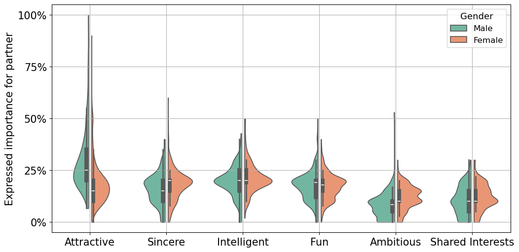
A first question one might ask is Are male and female participants interested in the same attributes for partner? To anwer it one can try and compare the reported importance to male and female candidates for partner characteristics (attractiveness, sincerity, intelligence, fun, ambition, shared interests). This is done by grouping the data associated to the columns : attr1_1, sinc1_1, intel1_1, fun1_1, amb1_1, shar1_1 by gender and then obtaining a violin plot. For context, this data is expressed as a set of weights for the six attributes that sum up to 100.
We observe in Figure 1 that in our dataset, on average males attribute a greater importance to physical attractiveness, while sincerity is more important to females. Moreover, some male participants attribute a great importance to attractiveness, sometimes close to 100%. On the other hand, both genders put a similar and low importance on ambition and having shared interests.
Successful vs. Unsuccessful candidates
In the previous paragaraph, some differences between male and female participants were outlined. Following this, it seems natural to wonder about the existance of differences within the same gender. One way to do this is to answer the question What are the differences between successful and unsuccessful female (respectively male)?
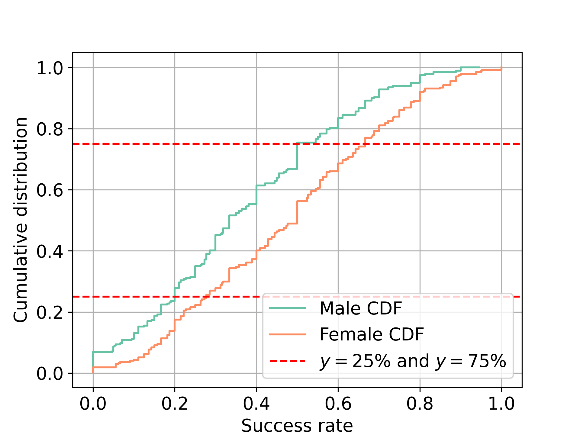
In order to give an answer, we use the fact that by the end of the experiment, each participant has recieved a certain number of “yes”s (grade: 1) and “no”s (grade: 0) by the partners they have met. This is contained in the column dec_o (decision of the other). We define the proportion of “yes”s each individual has recieved as a measure of their success. Notice that this measure will only take values between 0 and 1. On Figure 2 are represented the cumulative distributions of the success rate for male and female participants. These will allow us to categroize successful and unsuccessful individuals by looking at the intersection with the horizontal lines \(y=25\%\) and \(y=75\%\)
The curve representing male participants is shifted to the left compared to the one representing female ones. It can be deduced that males are on average less successful than females. The 25% least successful males are labeled in the following as “Unseccessful males” while the 25% most successful males are labeled as “Successful males”. Same definition holds for females.
In the sake of analyzing characteristics that differentiate successful and unsuccessful individuals, it is interesting to compare the interest each category (successful and unsuccessful) have, on average, for different activites. The interest for an activity has been expressed on a 1-10 scale. Data about the interest for 17 activties have been reported. Figure 3 and Figure 4 only report the results (for males and females respectively) for the five activities (reported in columns sports,tvsports,exercise,dining and clubbing)where the differences are statistically significant.
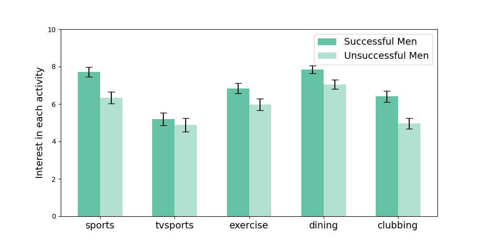
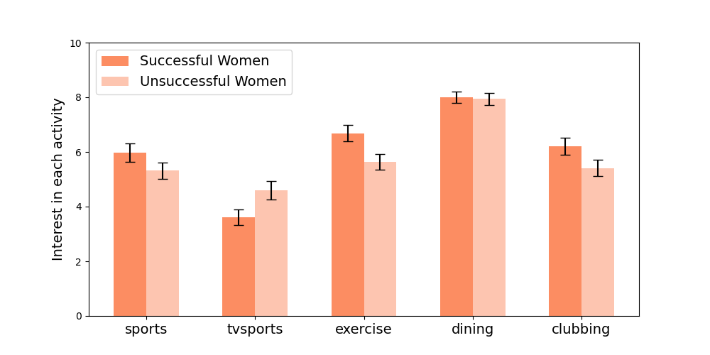
From the figure it can be observed that successful males have more interest for sports and exercice than unsuccessful males. Tvsports find more interest among unsuccessful females than successful ones. While successful and unsucessful female participants have the same interest for dining, successful males show a significant difference of interest compared to the unsuccessful ones. Both for male and female participants, clubbing recieves more interest from successful individuals (the difference is more marked for males).
Having analyzed the difference of interest for each activity there is between successful and successful male and female individuals, data regarding the rating (by the partners) of the attributes of each individual is analyzed in order to fully answer the question. Indeed, each participant recieves from their partners a grade (1-10 scale) on their percieved attributes (attractiveness, sincerity, intellect, fun and ambition). More precisely, for example, each male participant will recieve from each female participant a grade on how they look attractive. To each male will therefore be assigned an average grade on their attractiveness. An average over all successful males is then made. The same procedure is made for unsuccessful males, successful females and unsucessful females. The standard deviations of the data among each examined samples being similar and small enough (no standard deviation is greater than 0.14), it is more useful to deliver the data in tables. Table 1 shows the average grade recieved for each attribute for the 25% most successful and the 25% most unsuccessful males and female participants respectively.
| Quality | Successful Male | Unsuccessful Male | Successful Female | Unsuccessful Female |
|---|---|---|---|---|
| Attractiveness | 7.08 | 4.52 | 7.54 | 5.30 |
| Sincerity | 7.41 | 6.83 | 7.41 | 7.13 |
| Intellect | 7.72 | 7.18 | 7.53 | 7.02 |
| Fun | 7.28 | 5.06 | 7.19 | 5.77 |
| Ambition | 7.30 | 6.71 | 6.99 | 6.13 |
On average, successful individuals are more attractive, more sincere, more intelligent, more fun and more ambitous, be they males or females. It is worth noticing that unsuccessful females are on average given a grade of 5.30/10 for their attractiveness which is signficantly higer than the average grade given to unsuccessful males.
How much do shared interests really matter ?
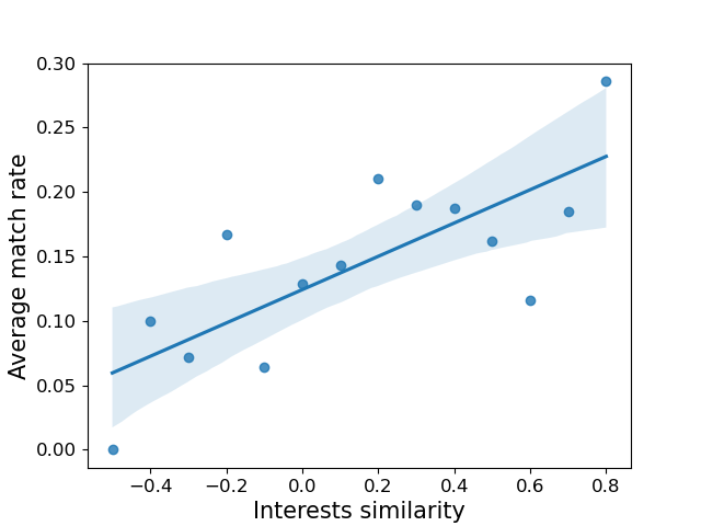
In the previous sections (Figure 1), we saw that participants overall declared putting a low importance on shared interests in the choice of partner. Surprised by this result, we wanted to shed light on How important are shared interests in matching? Exploring the data, one can find a int_corr variable, corresponding in the words of the authors to “correlation between participant’s and partner’s ratings of interests”. Thought this variable sounds promising to study impact of shared interest on compatibility, we were : 1. not able to make sense of it (i.e. re-derive the way in which it was obtained) 2. not able to obtain any sensible visualisation (the data looked like noise). Because of this we turned to the 1 to 10 grades that each participants associates to each of the 17 interests present in the dataset for help. By considering the grade vectors \(v_i\) and \(v_j\) for two candidates, we then defined the similarity between these through a scalar product as \[
S(v_i,v_j)=\frac{\langle\tilde{v}_i,\tilde{v}_j\rangle}{\|\tilde{v}_i\|\ \|\tilde{v}_j\|},
\]
where \(\tilde{v}_i={v}_i-5\) to recenter the vectors. Notice that this measure of similarity gives results in the \([-1,1]\) interval, with positive values associated to generally shared interests and negative ones with generally different interests.
Given this definition of similarity, one can then explore the effect of shared interests on the average match rate. This is done in Figure 5. The linear fit corresponds to an ordinary least squares linear regression. The shaded area is a 95% confidence interval that is estimated using a bootstrapping statistics, see NormandErwan (2018). By looking at it, one can easily see that there is a positive correlation between interest similarity and match rate.
Other notable factors
As mentionned previously, in addition to the data about prefered characteristics and interests, the used dataset contained a lot of personal information about the participants. Exapmples include age, field of study/work, SAT grade, income, religion and etnicity. In the following we explore the impact of some of this data.
Impact of SAT score on success rate
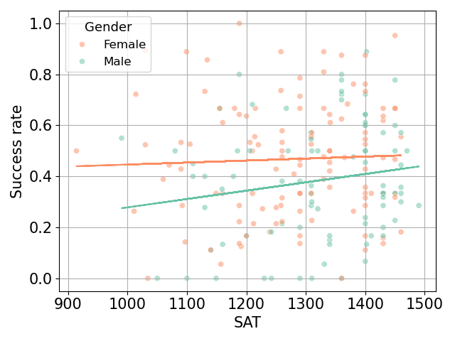
We would like to know if academic success is correlated with success in dating. To achieve this we use the SAT score included in the sat column of the dataset. While the SAT score is only used for university admissions, we’ll use it here a proxy metric for academic sucess. On the other hand, to quantify the success of participants, we will use the column dec_o \(\in {0, 1}\) indicating for each meeting if the participant was liked by the person in front of them. We define the success rate of participant \(i\) as the average of dec_o over all the speed dates in which \(i\) took part.
The first observation is that the average SAT score for men and women over the dataset are of 1320 and 1280 respectively, significantly higher than the national US average which is around 1050. Figure 6 contains a scatter plot of the success rate of male and female participants as a function of their SAT score. An ordinary least squares linear regression is associated to each gender. We observe a higher slope for males than females (\(3.3 \times 10^{-3}\) vs \(7.8 \times 10^{-5}\)), hinting that academic sucess is more important for men than women in speed dating success.
Impact of ethnicity on match
Wether it is because of habituation, people wanting to stay in their comfort zone or cultural influence, it is clear some people might prefer partners of their same ehnicity. Predicting the relation between stated importance and observed preference remains however untrivial. This is what we focus on in this section.
The relevant data to this section are the grades (on a 1-10 scale) that the participant attributed to the importance for their partner to be of the same ethnicity as them. The quantity we consider is the difference between the average acceptance of people of same ethnicity (which we call \(G_{ethn}\)) and the general one (which we call \(G_{all}\)). For the scale to be independent of the personal standards of the participants this difference is normalised by the acceptance rate of every individual. The average of \((G_{ethn}-G_{all})/G_{all}\) grouped by stated importance is plotted in Figure 7.
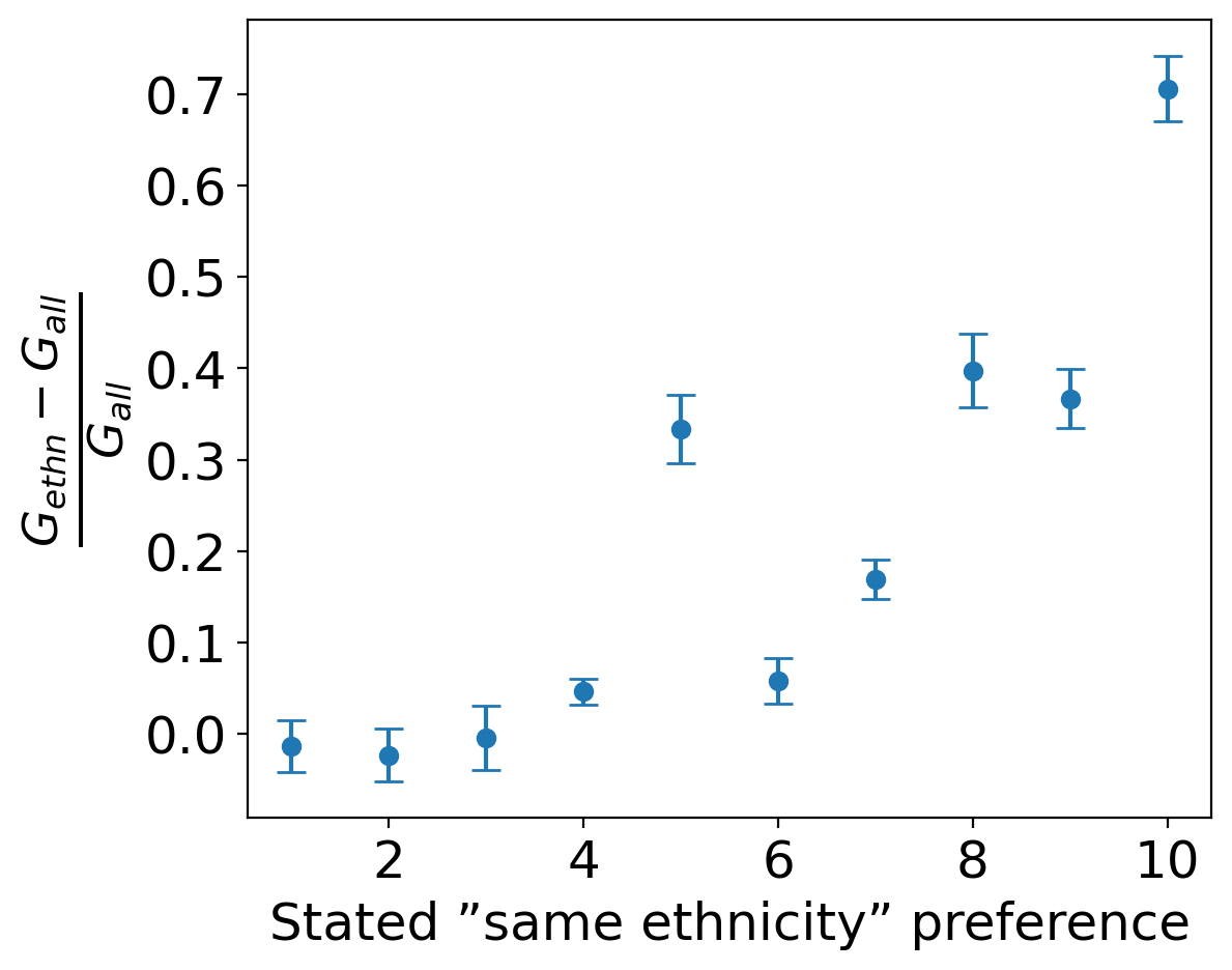
Looking at the figure it can be noticed that pople who stated a small importance (of 1,2 or 3 for example) for their partner to be of same ethnicity, indeed are (on average) associated to equal grading of the participants they met (the relative difference is close to zero). For people who state a bigger importance however, the relative difference seems to become significantly bigger than 0. People who reported a maximal importance to having a partner of the same ethnicity (10/10), are found to be 70% more likely to match with people of their ethnicity compared to others.
Do people percieve us as we do ?
As seen in the section about successful and unsuccesfull candidates, some factors, such as how fun and attractive people are, affect their successrate in speed dating. Given this observation, some might try to improve their chances of success by working on their shortcomings. This should be rather straight forward, assuming that person are able to gauge where they currenly stand. But is this a reasonable assumption? In this section we focus on investigating the relevance of this assumption.
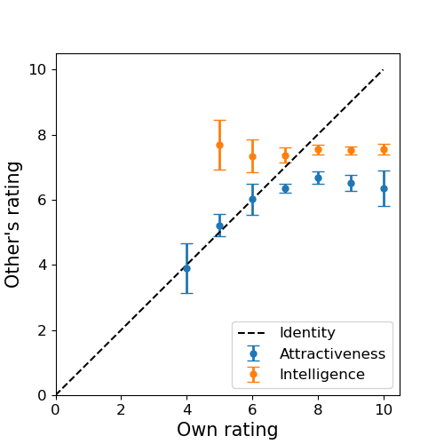
To do this we need to compare data about people’s own perception of themselves, and that of other people. Fortunately we have access to such data. Indeed, in addition to the attr, sinc, intel, fun, amb, shar ratings that other people give to the candidtes they meet, the dataset includes ratings that each person gave themselves on the same attributes. Figure 8 represents the self-prescribed ratings in terms of the externally prescribed ones. The values for the response variables were obtained by grouping the candidates by their self-prescribed ratings and taking the average. The confidence intervals correspond to \(\pm\hat{\sigma}\) where \(\hat \sigma\) is the corrected sample standard deviation. Notice that only the values associated to attractiveness and intelligence are included in order not to overcrowed the plot (the other attributes behaved similarly to intelligence anyway). A square-aspect ratio plot was chosen since the goal is to compare the observed results to the \(y=x\) baseline.
Looking at the figure, we immediately see that people’s own intelligence rating (on average) does not correlate with other people’s ratings. This might sound surprising at first. It can however be understood by noticing that intelligence is a vague term, which makes it is hard to evaluate both your own rating and evaluate that of someone else. In the second case, this is aggraveted by the fact that the estimate is only based on a 4 minute interraction. The observed behaviour for attractiveness is more nuanced. On one hand, it seems that people are (on average) good at evaluating when they do not appear attractive to others. This is reflected by the fact that the points associated to the 4,5,6 ratings nicely overlap with the \(y=x\) line. On the other hand, there is no significant difference in externally-reported attractiveness between groups that self-report their attractiveness as 7,8,9 or 10 out of 10. The only difference between these groups seems therefore to be in their ego.
Conclusion
In conclusion, the exploration of the Speed dating dataset from Fisman’s 2006 study has provided valuable insights into the dynamics of modern dating within a fast-paced society. This analysis has shed light on several key aspects of speed dating, including partner preferences, gendered differences, shared interests, and ethnicity influences on compatibility.
One notable finding from this investigation is the existence of gendered differences in partner’s attributes preferences. Most successful and most unsuccessful individuals show a neat difference in some interest for a certain type of actvities (such as doing sports of clubbing), as well as a difference in their attributes.
Moreover, the role of shared interests and ethnicity preferences in shaping compatibility has been highlighted. The data suggests that common interests play a significant role in forming connections during brief encounters.
In essence, the Speed dating dataset analysis has underscored that love and romantic connections can be influenced by a complex interplay of factors. While the findings of this study are intriguing and hold practical implications, it is essential to remember that they represent statistical insights, and the genuine power of love between two individuals transcends mere statistics.